Overview
During the downtime due to the pandemic-inspired shelter-in-place in California, I’ve decided to learn some new technologies and concepts related to software design. This has been my first foray into online learning using one of the e-learning platforms. In this case, I signed up for Udacity (https://www.udacity.com).
So far, I’ve been quite impressed. Of course, it does not perfectly substitute live classroom instruction, but it is still quite effective, plus I can skip to the good parts. The course I signed up for is titled “Artificial Intelligence and Python”.
While I’ve programmed scripts with Python before, I never knew that it had some many math and statistic-intensive libraries. Hence, it’s a great language for developing AI-related software since AI is all about statistics: predicting future events based upon historical information.
While the basics of Python programming is not that interesting, the libraries and tools associated with Python are fascinating and actually lots of fun to work with. This blog post will talk a bit about those libraries and also how they apply to AI. As of mid-April 2020, I have not finished the course yet, so emphasis is on the Python libraries used for AI, but not quite AI, itself.
NumPy
NumPy is a library for Python. It is short for “Numerical Python”, and it includes a large amount of functionality related to multi-dimensional arrays and matrices in addition to many mathematical functions. Users can create arrays from Python dictionaries, and then manipulate the arrays in many different ways including reshaping arrays, adding arrays, multiplying arrays, and much much more.
Here’s an example of how a simple numpy array works in Python:
1. import numpy as np
2. x = np.array([0,1,2,3,4,5,6,7,8,9])
3. print(x)
4. [0 1 2 3 4 5 6 7 8 9 10]
Line 1 imports the numpy library and renames it.
Line 2 defines a single row array with values from 0 to 9.
Line 3 prints the array and Line 4 displays it.
Let’s take it a step further:
5. x.reshape(2,5)
6. print(x)
7. [[0,1,2,3,4]
[5,6,7,8,9]]
Line 5 executes the “reshape” function that changes the shape of the array from a single row to a 2×5 array as seen in Line 7.
Other functions allow you to insert rows in an array:
8. x = np.insert(x, 1, [10,11,12,13,14], axis=0)
The above “insert” statement inserts a new row at row 1 (row numbers start at 0). The numbers it inserts are: 10,11,12,13,14. The “axis” tells whether to insert a row (0) or column (1).
You can also perform mathematics on 2 arrays including addition, subtraction, multiplication, and division. For example:
x = [[0,1,2,3,4]
[5,6,7,8,9]]
y = [[6,3,2,8,7]
[1,6,7,3,10]]
print(x + y) = [[6,4,4,11,11]
[6,12,14,11,19]]
The above “x” adds each of the elements from each row and column and creates the corresponding matrix with the added values. You can also do the same with the other mathematical functions.
There are many functions associated with numpy that can be found in lots of online documentation.
Pandas
Pandas is another Python library that deals with data analysis and manipulation. It takes the numpy arrays one step further and allow the creation of complex arrays. Let’s look at an example:
- import pandas as pd
- groceries = pd.Series(data=[30,6,’Yes’,’No’], index=[‘eggs’,’apples’,’milk’,’bread’])
Line 1 imports the Pandas library. Line 2 creates a complex matrix where the first column is the index of labels and the 2nd column is the actual data. It looks like this:
| eggs | 30 |
|---|---|
| apples | 6 |
| milk | Yes |
| bread | No |
dtype: object
If you “print groceries[‘eggs’]”. The result is: 30.
Pandas allows you to perform mathematics on values in a matrix:
print(groceries / 2) =
| eggs | 15 |
|---|---|
| apples | 3 |
| milk | Yes |
| bread | No |
You can also create a more complex matrix by creating a dictionary of Pandas series:
3. items = {‘Bob’ : pd.Series(data = [245, 25, 55], index = [‘bike’, ‘pants’, ‘watch’]),
‘Alice’ : pd.Series(data = [40, 110, 500, 45], index = [‘book’, ‘glasses’, ‘bike’, ‘pants’])}
4. shopping_carts = pd.DataFrame(items)
5. shopping_carts
| Bob | Alice | |
|---|---|---|
| bike | 245.0 | 500.0 |
| book | NaN | 40.0 |
| glasses | NaN | 110.0 |
| pants | 25.0 | 45.0 |
| watch | 55.0 | NaN |
shopping_carts[‘Bob’][‘Bike’] displays “245.0”.
You can also create a Python dictionary and then create a Panda dataframe from the dictionary along with indexes. See the following:
#Create a list of Python dictionaries
items2 = [{‘bikes’: 21, ‘pants’: 36, ‘watches’: 40}, {‘watches’: 12, ‘glasses’: 51, ‘bikes’: 18, ‘pants’:9}]
#Create a Panda DataFrame
store_items = pd.DataFrame(items2, index=[‘store 1’, ‘store 2’])
#Display the DataFrame
store_items
It displays as:
| bikes | pants | watches | glasses | |
|---|---|---|---|---|
| store 1 | 20 | 30 | 35 | NaN |
| store 2 | 15 | 5 | 10 | 50.0 |
To add a column:
store_items[‘shirts’] = [15,2]
Now, the DataFrame displays:
| bikes | pants | watches | glasses | shirts | |
|---|---|---|---|---|---|
| store 1 | 20 | 30 | 35 | NaN | 15 |
| store 2 | 15 | 5 | 10 | 50.0 | 2 |
Anaconda and Jupyter Notebooks
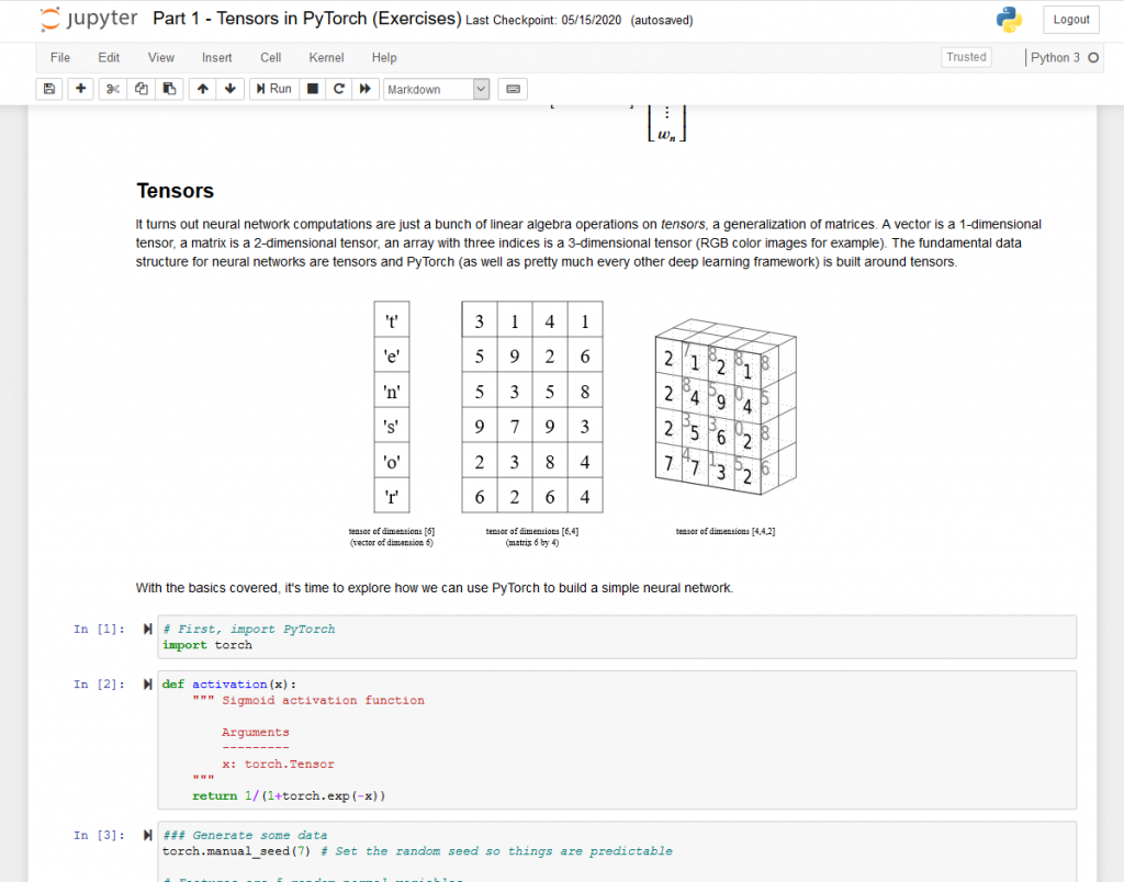
Now that I have covered a bit of NumPy and Pandas for manipulating data arrays, let’s delve a bit into a Python platform called Anaconda. Anaconda is a “navigator” that allows users to download any and all libraries available for the Python platform. These libraries include mathematical libraries, different types of Python compilers, artificial intelligence libraries (like PyTorch) and the Jupyter Notebook which is a web-based user interface for displaying comments and typing in Python code that runs on command. It’s a tool not necessarily to write production-level Python code, but more a tool to train and test out python code while displaying well-formatted comments.
Below is an example of a Jupyter webpage (or notebook) that includes a comments section with images and then a subsequent code section. This Jupyter notebook talks about Python tensors and Pytorch, the essentials for artificial intelligence.
Neural Networks
Neural networks have been around for a while. The basically emulate the way our brains work. The networks are built from individual parts approximating neurons which are interconnected and are the basis for how the brain learns.
“Digital” neurons are no different. They are interconnected in such a way that over time they learn and are able to apply the learned knowledge to enable useful applications such as natural language (like Alexa) and image identification (like Google Lens). It really is amazing how well it works, and the progress over the past five years alone has been remarkable. I’ll talk more about that later.
So how does it work exactly? Let’s take the example of identifying text in an image; specifically, digits 0 to 9. Just 5 years ago, this was a very complicated problem. Today, it’s a trivial one. The image below displays greyscale handwritten digits where each image is 28×28 pixels.
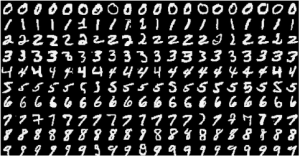
Greyscale handwritten digits
The first step is to train the software or the “network” in AI lingo. This means feeding it 100s if not 1000s of sample 28×28 pixel images of digits and tagging those images with the actual numbers so the software learns what number the image represents exactly. Luckily, Pytorch includes lots of tagged training data called MNIST. This data can be used to train the network so when you present your own image of a digit, it will correctly interpret what it is.
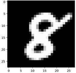
Single digit
The above image is an example of a greyscale “8” that is 28 x 28 pixels. This is the type of image that would be fed into the network to train it that this type of image is an “8”.
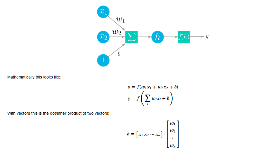
Neural Networks
The above images shows a simple neural network. The far left-hand side displays the inputs (x1 and x2). In our example, the inputs would be the color of each of the 28 x 28 pixels. The values (w1 and w2) are called “weights” These weights are multiplied by each of the corresponding inputs (i.e. – dot product of two vectors) and then inputted into a function that creates an output value (0 to 9) that is compared to the actual value assigned to the image. For example, in the digit training image above (the number “8”), the tag assigned to this image is 8. Therefore, the calculated output is compared to the tagged value. If it matches, then we’ve trained it well for that particular test image and the weights will be reused. If not, then we need to go back and adjust the weights to create a new output value. This back and forth can occur 1000s of times until the correct formula is found.

