In June of 2020, Carmel Software received a U.S. Department of Energy Small Business Innovation Research (SBIR) grant to develop a new software tool to help energy modelers and energy auditors better design and maintain energy efficient buildings. The details of that grant were detailed in a prior blog post. This blog post will detail the progress that we have made so far. First, we need to restate the problem that has become even more urgent since last year:
As part of its national infrastructure plan, the Biden Administration has set a goal to retrofit 2 million commercial and residential buildings over the next 4 years. Energy usage and energy auditing data for these buildings need to be stored in a consistent manner to help achieve this aggressive goal.
Simulating the energy usage of buildings using sophisticated software has become a key strategy in designing high performance buildings that can better meet the needs of society. Automated exchange of data between the architect’s software design tools and the energy consultant’s simulation software tools is an important part of the current and future building design process.
In the Phase I funding opportunity announcement (ie – request for proposal or “FOA”), the DOE’s Building Technology Office (BTO) was asking that bidders suggest new workflows for either BuildingSync or HPXML, which are schema “languages” that allow for the transfer of commercial and residential energy auditing information, respectively . Our proposal focused on BuildingSync XML since we are more focused on the commercial building market. Phase I of this proposal focused on the workflow that involves the U.S. Department of Energy’s Asset Score Audit Template to BuildingSync to the ASHRAE Building EQ benchmarking portal. Carmel Software successfully developed a beta of Schema Server that streamlines the flow of information from DOE’s Asset Score Audit Template into ASHRAE Building EQ. With the simple click of a button, the producing or consuming tool performs quick data checks, tests-case validations, and then transfers to the consuming tool (in this case, ASHRAE Building EQ). We also integrated a gbXML viewer and validator so that any accompanying gbXML file for the same building as the BuildingSync XML file could be validated and viewed (assuming it includes the building’s 3D geometry designed from a tool like Autodesk Revit). We also went a bit beyond the scope of the original proposal and added the following features based upon user feedback:
We incorporated building data from additional data sources, most importantly from Energy Star Portfolio Manager. We are now able to import monthly and yearly building utility data (for electricity, natural gas, and other fuel types). This data is used by ASHRAE Building EQ to calculate the Building EQ Score. We do this by integrating with the Energy Star PM API (application programming interface).
We talked with many energy auditors and all of them use Excel to tabulate data and create reports. We created an integration with Microsoft Office software including Word and Excel. This integration allows users to create customized Office templates with keycodes representing data types from the BuildingSync XML data schema. This, in turn, will populate these customized Office templates with actual data from the BuildingSync XML files. The benefit of this is it allows users to keep their custom reporting Excel templates and populate them with data imported by Schema Server.
When we presented the Phase I beta to our DOE program manager and other interested parties, they were quite pleased with the progress that we have made so far. Most importantly, we began validating the true purpose and use of this portal by talking with 50 stakeholders over a 6-month period. The following objectives were outlined in Phase I and were met (or will be met by the end of the Phase I time-period of May 31, 2021):
Objective 1: RPI identified 10+ candidate test cases by interviewing energy modeling practitioners and other related professionals to identify issues with the current building asset data to consuming software tool workflow.
Objective 2: Selected the seven (7) or so most important test cases.
Objective 3: Developed the Schema Server web portal that included the functionality described above.
Objective 4: Developed an application programming interface (API) that allows third-party software developers to integrate with the Schema. This currently only works with Audit Template and Building EQ but will be expanded during Phase II.
We developed Schema Server (https://www.schemaserver.com) which incorporates many of the objectives listed above. This website allows users to create an account, add projects, import BuildingSync XML schemas from Audit Template, validate those schemas, export to ASHRAE Building EQ. It even allows you to store multiple versions of the BuildingSync XML file so it simulates a sort of version control software.
Let’s look at some of the functionality of this website. You are able to create a free account that allows you to begin entering as many projects as you want. A “project” is usually a building.
You can enter the following information about a building including basic demographic information:
We’ll discuss the Energy Star options later. At the bottom of this page is the “Schema Version List”. This is a list of all of the schema file uploads for this particular project. Think of it as almost a version control list similar to GitHub where it includes a list of all of the changes made on one or more files. This Schema Version List is a list of all of the changes that you have made to a schema file (either Building Sync XML or gbXML or others in the future).
As the user adds new schemas to the list, the version number automatically increases. When the user clicks one of the rows, it directs the user to a new web page that appears as follows:
Clicking the Validate button performs validation on the BuildingSync file using what is called Schematron. Schematron is used for business rules validation, general validation, quality control, and quality assurance that is that allows users to develop software-specific validation modules. The SchemaServer Schematron produces a report listing mandatory fields that are missing and a list of generic errors in relation to the imported BuildingSync file. The screenshot below shows an example of this:
The View button takes the user to a new webpage that allows the user to view the XML file in different ways:
During the downtime due to the pandemic-inspired shelter-in-place in California, I’ve decided to learn some new technologies and concepts related to software design. This has been my first foray into online learning using one of the e-learning platforms. In this case, I signed up for Udacity (https://www.udacity.com).
So far, I’ve been quite impressed. Of course, it does not perfectly substitute live classroom instruction, but it is still quite effective, plus I can skip to the good parts. The course I signed up for is titled “Artificial Intelligence and Python”.
While I’ve programmed scripts with Python before, I never knew that it had some many math and statistic-intensive libraries. Hence, it’s a great language for developing AI-related software since AI is all about statistics: predicting future events based upon historical information.
While the basics of Python programming is not that interesting, the libraries and tools associated with Python are fascinating and actually lots of fun to work with. This blog post will talk a bit about those libraries and also how they apply to AI. As of mid-April 2020, I have not finished the course yet, so emphasis is on the Python libraries used for AI, but not quite AI, itself.
NumPy
NumPy is a library for Python. It is short for “Numerical Python”, and it includes a large amount of functionality related to multi-dimensional arrays and matrices in addition to many mathematical functions. Users can create arrays from Python dictionaries, and then manipulate the arrays in many different ways including reshaping arrays, adding arrays, multiplying arrays, and much much more.
Here’s an example of how a simple numpy array works in Python:
Line 1 imports the numpy library and renames it. Line 2 defines a single row array with values from 0 to 9. Line 3 prints the array and Line 4 displays it.
Line 5 executes the “reshape” function that changes the shape of the array from a single row to a 2×5 array as seen in Line 7. Other functions allow you to insert rows in an array:
8. x = np.insert(x, 1, [10,11,12,13,14], axis=0)
The above “insert” statement inserts a new row at row 1 (row numbers start at 0). The numbers it inserts are: 10,11,12,13,14. The “axis” tells whether to insert a row (0) or column (1).
You can also perform mathematics on 2 arrays including addition, subtraction, multiplication, and division. For example:
x = [[0,1,2,3,4] [5,6,7,8,9]]
y = [[6,3,2,8,7] [1,6,7,3,10]]
print(x + y) = [[6,4,4,11,11] [6,12,14,11,19]]
The above “x” adds each of the elements from each row and column and creates the corresponding matrix with the added values. You can also do the same with the other mathematical functions.
There are many functions associated with numpy that can be found in lots of online documentation.
Pandas
Pandas is another Python library that deals with data analysis and manipulation. It takes the numpy arrays one step further and allow the creation of complex arrays. Let’s look at an example:
Line 1 imports the Pandas library. Line 2 creates a complex matrix where the first column is the index of labels and the 2nd column is the actual data. It looks like this:
eggs
30
apples
6
milk
Yes
bread
No
dtype: object
If you “print groceries[‘eggs’]”. The result is: 30.
Pandas allows you to perform mathematics on values in a matrix:
print(groceries / 2) =
eggs
15
apples
3
milk
Yes
bread
No
You can also create a more complex matrix by creating a dictionary of Pandas series:
You can also create a Python dictionary and then create a Panda dataframe from the dictionary along with indexes. See the following:
#Create a list of Python dictionaries items2 = [{‘bikes’: 21, ‘pants’: 36, ‘watches’: 40}, {‘watches’: 12, ‘glasses’: 51, ‘bikes’: 18, ‘pants’:9}]
#Create a Panda DataFrame store_items = pd.DataFrame(items2, index=[‘store 1’, ‘store 2’])
#Display the DataFrame store_items
It displays as:
bikes
pants
watches
glasses
store 1
20
30
35
NaN
store 2
15
5
10
50.0
To add a column:
store_items[‘shirts’] = [15,2]
Now, the DataFrame displays:
bikes
pants
watches
glasses
shirts
store 1
20
30
35
NaN
15
store 2
15
5
10
50.0
2
Anaconda and Jupyter Notebooks
Now that I have covered a bit of NumPy and Pandas for manipulating data arrays, let’s delve a bit into a Python platform called Anaconda. Anaconda is a “navigator” that allows users to download any and all libraries available for the Python platform. These libraries include mathematical libraries, different types of Python compilers, artificial intelligence libraries (like PyTorch) and the Jupyter Notebook which is a web-based user interface for displaying comments and typing in Python code that runs on command. It’s a tool not necessarily to write production-level Python code, but more a tool to train and test out python code while displaying well-formatted comments.
Below is an example of a Jupyter webpage (or notebook) that includes a comments section with images and then a subsequent code section. This Jupyter notebook talks about Python tensors and Pytorch, the essentials for artificial intelligence.
Neural Networks
Neural networks have been around for a while. The basically emulate the way our brains work. The networks are built from individual parts approximating neurons which are interconnected and are the basis for how the brain learns.
“Digital” neurons are no different. They are interconnected in such a way that over time they learn and are able to apply the learned knowledge to enable useful applications such as natural language (like Alexa) and image identification (like Google Lens). It really is amazing how well it works, and the progress over the past five years alone has been remarkable. I’ll talk more about that later.
So how does it work exactly? Let’s take the example of identifying text in an image; specifically, digits 0 to 9. Just 5 years ago, this was a very complicated problem. Today, it’s a trivial one. The image below displays greyscale handwritten digits where each image is 28×28 pixels.
Greyscale handwritten digits
The first step is to train the software or the “network” in AI lingo. This means feeding it 100s if not 1000s of sample 28×28 pixel images of digits and tagging those images with the actual numbers so the software learns what number the image represents exactly. Luckily, Pytorch includes lots of tagged training data called MNIST. This data can be used to train the network so when you present your own image of a digit, it will correctly interpret what it is.
Single digit
The above image is an example of a greyscale “8” that is 28 x 28 pixels. This is the type of image that would be fed into the network to train it that this type of image is an “8”.
Neural Networks
The above images shows a simple neural network. The far left-hand side displays the inputs (x1 and x2). In our example, the inputs would be the color of each of the 28 x 28 pixels. The values (w1 and w2) are called “weights” These weights are multiplied by each of the corresponding inputs (i.e. – dot product of two vectors) and then inputted into a function that creates an output value (0 to 9) that is compared to the actual value assigned to the image. For example, in the digit training image above (the number “8”), the tag assigned to this image is 8. Therefore, the calculated output is compared to the tagged value. If it matches, then we’ve trained it well for that particular test image and the weights will be reused. If not, then we need to go back and adjust the weights to create a new output value. This back and forth can occur 1000s of times until the correct formula is found.